Smarter Road Logistics

Efficiency in Road Logistics

For thousands of years, it was sufficient for merchants to rely on experience and intuition when transporting their goods, but this has changed. In 2016, 2200 Billion tonne-kilometers of goods were transported in Europe alone, 75% of which on roads. Now imagine, you are driving on one of these roads and there is a truck in front of you. What is your estimate about the probability of that truck being empty? For Austria, the correct answer would be 50%. Half of all tours are empty. This is not just an economic problem — for operating companies and for people stuck in traffic congestions — but it is also harmful for the environment. In a small example, we will show, how a modern toolset of different technologies can help us to make better decisions, leading to more efficient and sustainable transportation.

Planning Schedules in Logistics

First of, you might ask yourself: How is that even possible? After all, it costs a lot of money to drive empty trucks around. Taking Austrian numbers from Eurostat, empty hauls cost transport providers about 945M€ per year². For margin businesses, this is a lot of money. So why haven't there been larger investments in technologies that aim to solve these problems and what prevents transportation providers from being more efficient with their resources?

Without giving away any internal details, I can confirm many of the problems that have often been discussed in common logistics literature. Transportation processes are vastly complex and coordination depends on many external, unpredictable factors. Thus, lots of planning happens manually or using dedicated software, that specializes on one particular aspect of transportation, but does not integrate well with other software.

Let us start by picking one typical mode of transportation, which is also a large part of the businesses of DB Schenker and similar logistics providers: Less-than-truckload (LTL) shipping. With LTL shipping, the freight is moved through a network of hubs using scheduled tours and turnovers before being delivered to the customer. DB Schenker operates such an LTL network with eleven turnover nodes in Austria. It is their job to schedule all trucks within the network, which are a couple of hundred movements per week. The schedule needs to ensure that there are enough connections for fast transportation, while keeping vehicles well utilized. The state-of-the-art approach to planning schedules is strategic: schedules are only updated a couple of times each year, which means that planning depends on long-term forecasts and cannot predict changes in short-term demand. If planning were to become more flexible, these fluctuations could be considered, potentially leading to more efficient transportation.

Automizing Scheduling Decisions

As a first step towards more flexible schedules, our aim was to design a system that adapts vehicle schedules autonomously, based on current demand. This required us to do three things: (1) monitor the current network state, (2) calculate adaptions to the schedule and (3) construct a mechanism that can react to unforseen delays. I will cover all three parts in the following sections.

Part 1: Collecting Data in Real Time

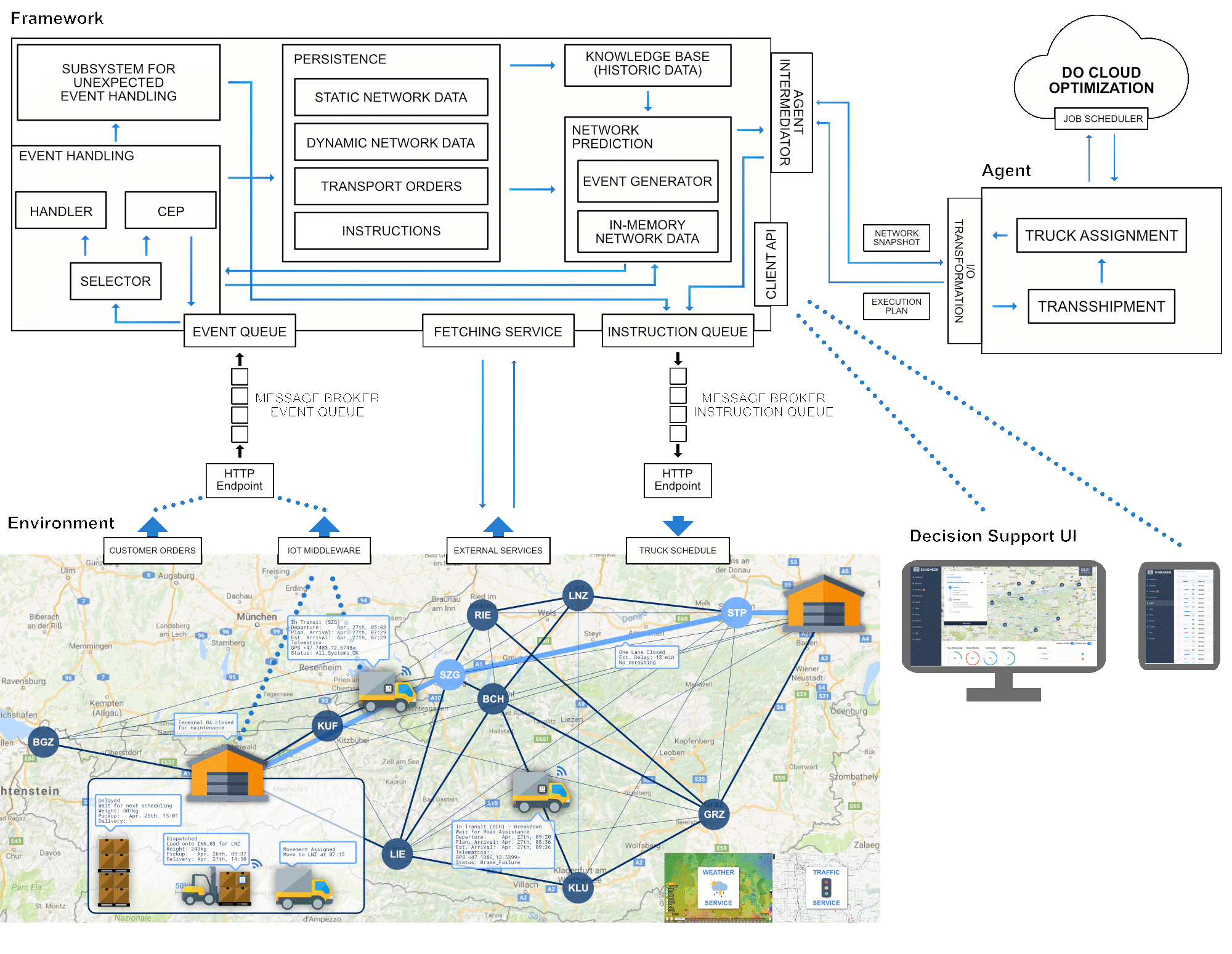
In the figure below, you can see a diagram of the application architecture we designed to collect all the required data. This allows us to monitor freight and vehicle movements in a transportation network, including the status and location of shipments via RFID or barcodes, the location of vehicles with telemetry data and GPS, current travel times on calculated routes via the Google Road API and current weather information from the Weather Company. We use event processing to mould these events into a single, coherent digital image of the network to provide uniform access to all participating entities and items.

Part 2: Calculating Dynamic Vehicle Schedules

Based on the observations we have from Part 1, we can automatize some of the decision processes related to schedule planning. In principle, this means answering the following question:

Given a logistics network with turnover hubs and transportation vehicles and a set of shipments at their origin node, what is the optimal way to move them to their destination? How many vehicles are required, when are they scheduled and which routes do they take?

As it turns out, there already exists a formalized problem that loosely models our case with LTL shipping. It is called the Transshipment Problem ³ and we can use it as a starting point to add further constraints. The Transshipment Problem is an optimization problem, consisting of a set of hubs $H$, a set of shipments $balance$, which contains the weights, origins and destinations for all shipments and three matrices: the distance matrix $d$, which contains the distances between all nodes and the two decision matrices $s$ and $v$, where $s$ determines the route of shipments through hubs and $v$ assigns a number of vehicles to each connection in $d$, based on $s$.

The objective of the problem is to minimize the overall distances driven by all vehicles:

A constraint ensures that shipments depart from their origin and arrive at their destination. Another constraint limits the capacity of each hub $capacity_h$. Finally, we use a third constraint to limit the capacity of vehicles $capacity_v$.

To better model our given problem, we need to extend the Transshipment Problem with a number of dimensions and constraints:

1. Time: No schedule can exist without time, which is why we need to add a discrete dimension for time.
2. Temporal Constraints:These constraints account for travel times and times for loading and unloading.
3. Moving Vehicles: The traditional problem considers vehicles a static resource, but in real logistics networks, vehicles are moving all the time. This means that vehicles that are available now, might not be available the next day at the same location.
4. Memory: Since our calculations alter an existing plan, we need to be able to incorporate previous schedules into current calculations. This is in contrast to the traditional problem, where each solution is calculated from scratch. Conveniently, we can use the same mechanism to include data such as long-term forecasts into the caluclation.

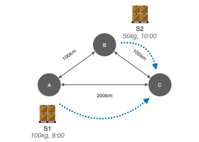
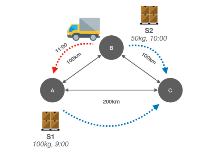
These three scenarios give you an overview of the goal of our calculations. Each scenario results in a schedule that is depicted in the table below each scenario. Note that the third scenario includes a movement from a previous calculation.

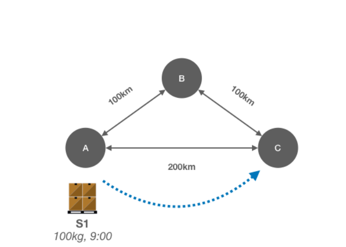
FROM	TO	TRUCK	DEP	ARR	SHIP
A	C	1	10	12	S1

FROM	TO	TRUCK	DEP	ARR	SHIP
A	B	1	10	11	S1
B	C	1	12	14	S1,S2

FROM	TO	TRUCK	DEP	ARR	SHIP
B	A	0	11	12	SS
A	C	1	13	15	S1,S2

The last thing we need to do in order to calculate complete schedules is vehicle assignments. So far, we only computed where and when how many vehicles should be driving. We did not say who should be driving. Our second optimization model for Vehicle Assignment finds a solution for that.

Part 3: Handling Unexpected Delays

Since our system directly interferes with daily operations, it needs to be aware of incidents that cause delays, in case the actual plan no longer works. It also needs to provide a context-aware mechanism for resolving such incidents. We came up with a categorization that knows three types of events that cause delays:

1. Single Vehicle: If one vehicle is involved, e.g., technical breakdowns
2. Single Connection: If one connection is affected, e.g., traffic congestions
3. Multi Connection: If multiple connections are affected, e.g., bad weather conditions

Part 4: Demo User Interface

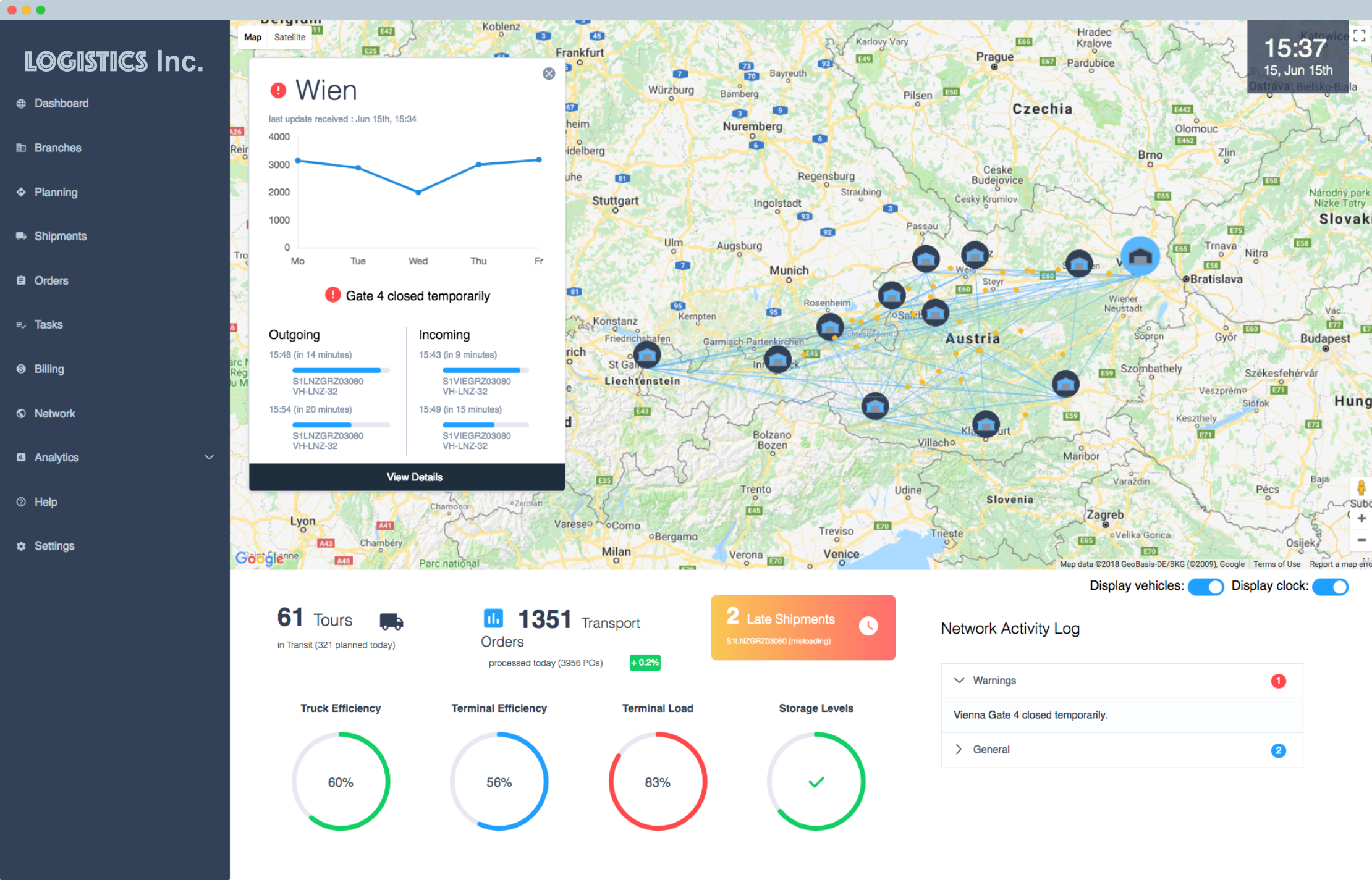
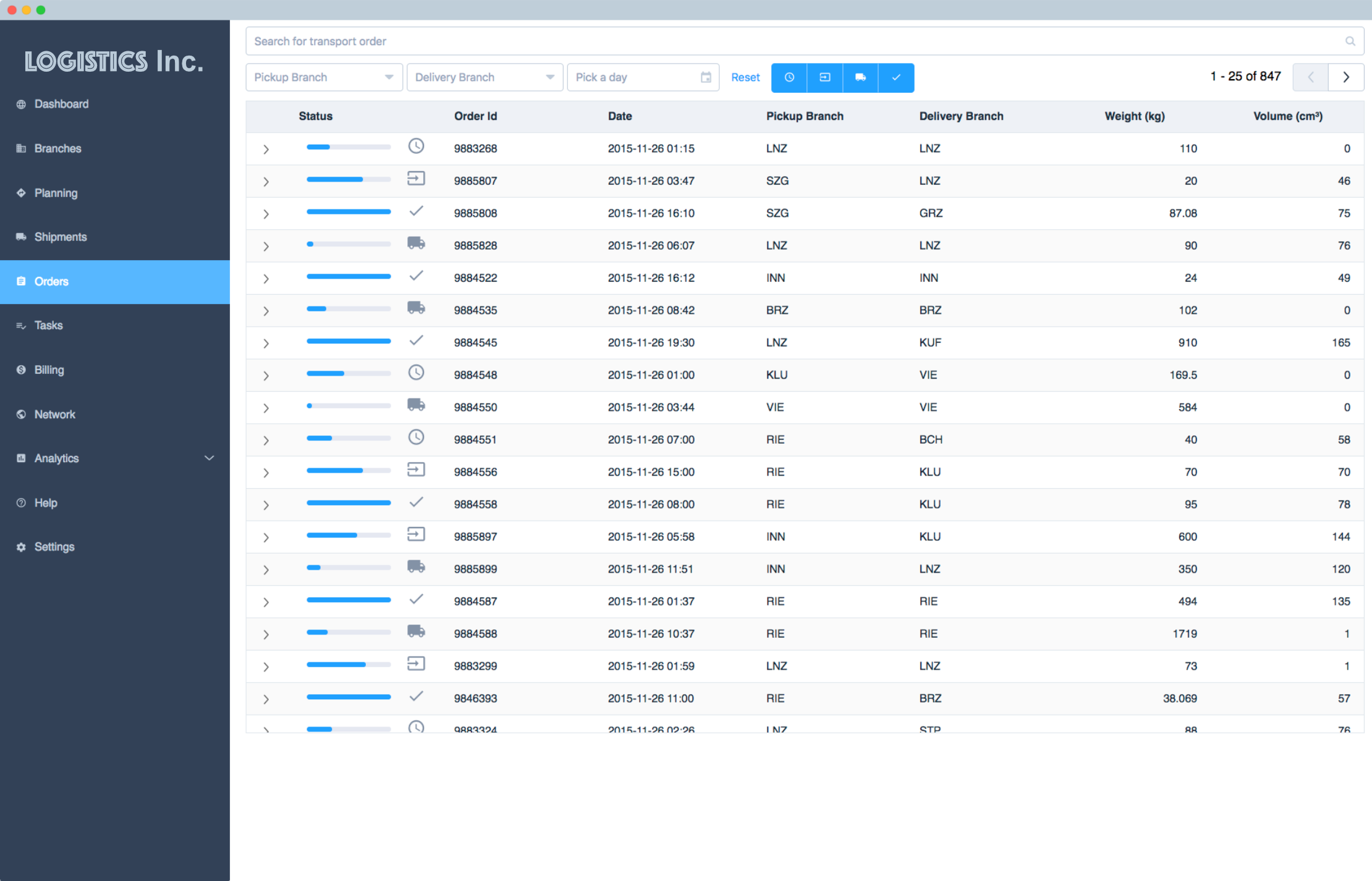
For show-cases and demos, we designed a UI that visualizes the current network state and provides some statistics on performance indicators.

Experiments

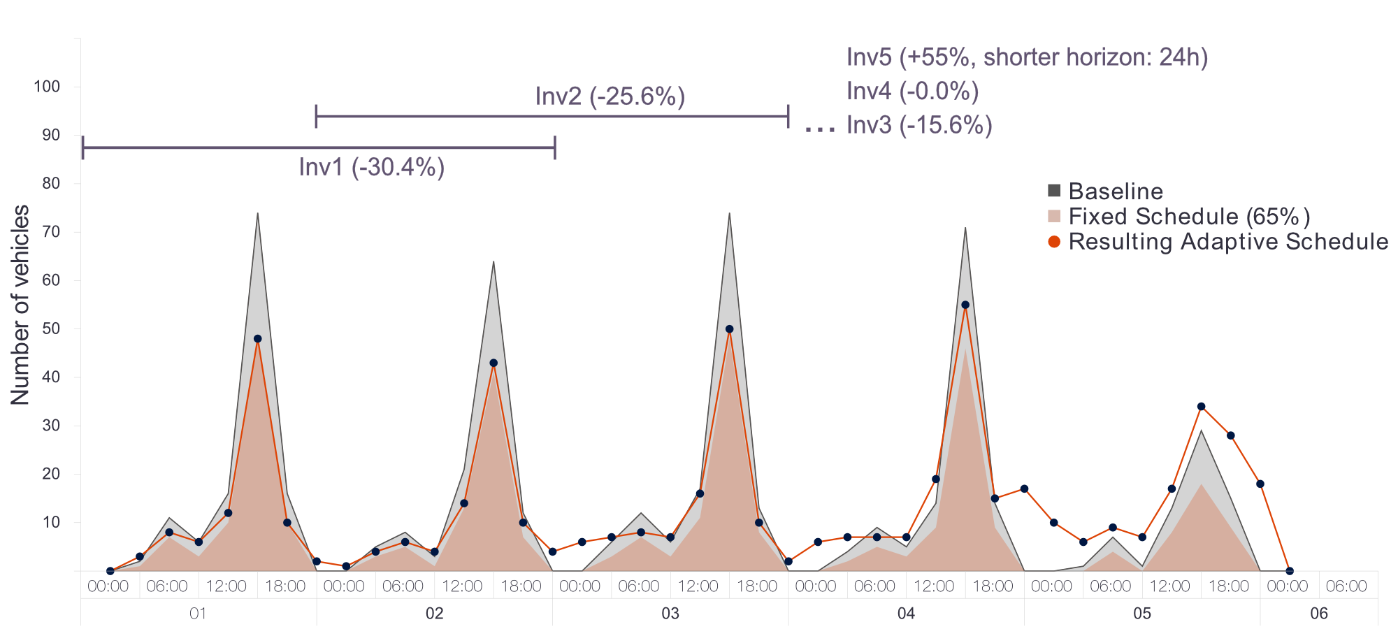
The figure below depicts the history from one of our simulations, which simulated one week of network activity. In the graph you can see a grey area, which represents the traditional, fixed schedule and a red-dotted line, which represents the dynamic schedule, calculated by our models. Each invocation of schedule optimizer is marked as Inv (1-5). In this particular experiment, we assumed that 65% of the movements from the fixed schedule would be included into our calculations. This simplified calculations and brought more stability to the overall schedule. In general, there is a lot to say about the results, but the most noticable difference lies in the balance of resources: In the beginning of the week, our approach requires much less resources, while at the end of the week, it uses more.

Results

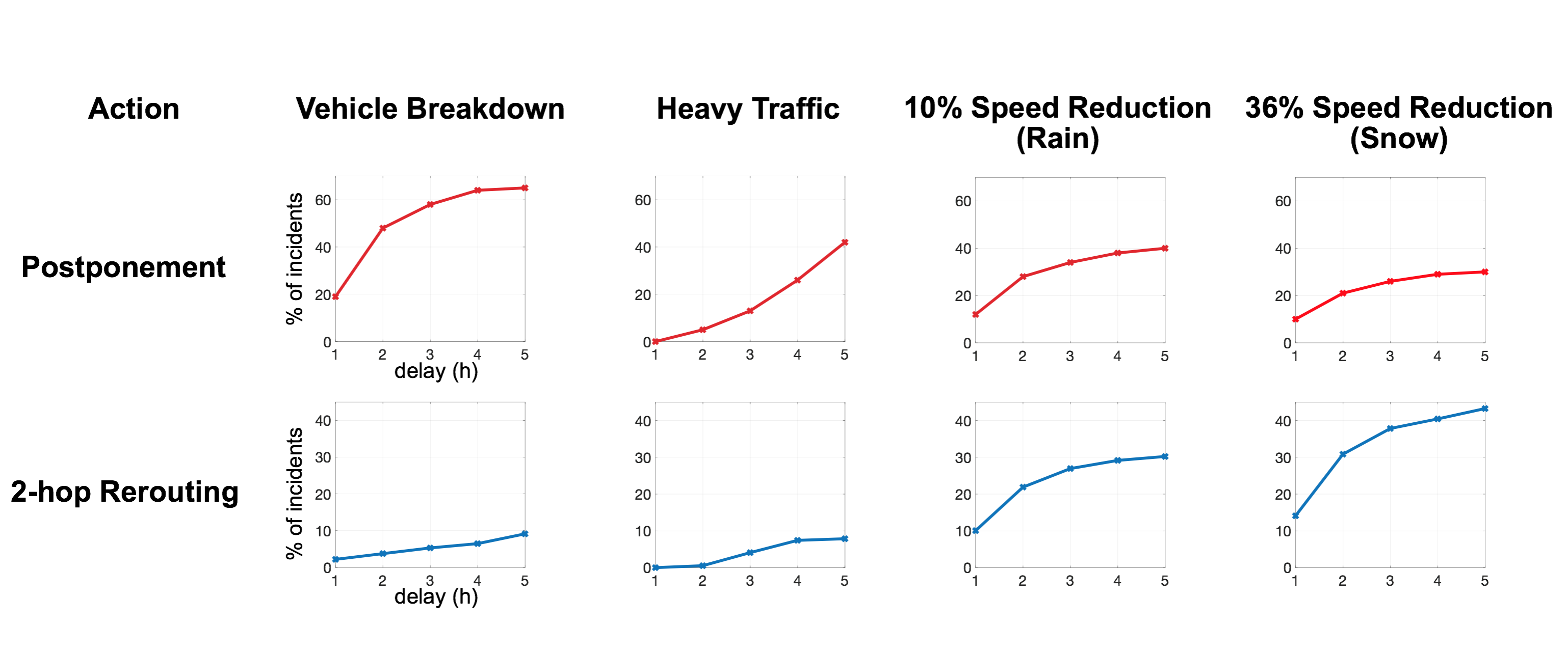
Overall, our tool managed to improve the schedule by using 2.01% less movements, improving vehicle utilization by 2.8 percentage points and reducing the overall amount of driven kilometers by 15.6%. In a second line of experiments, we tested the impact of unforeseen incidents on the schedule. Overall, we saw that most of the single vehicle delays required postponement of future tours, while multi connection delays often required a rerouting of shipments, as simple postponement was not sufficient. In the first case, an average 1.15 vehicles were affected per incident. This number grew to 3.5 with multi connection delays.

Summary

To summarize all of the above: There are too many empty trucks on the road. We thought about how to solve this problem and came up with a technical solution for LTL logistics providers. With our solution, we aim to improve the efficiency of schedules by monitoring the current network state and adapting schedules on-demand. In our simulations, we were able to reduce the amount of driven kilomers by 15.6%, marking considerable improvements.

Notes and References

1. Statistics about road freight transportation in the EU, published by Eurostat, 2016 (Link to Publication)
2. Take 25 Billion tonne-kilometers per year and an average load of 14 tons per transport (both Eurostat numbers for Austria), which leaves us with 1.8 Billion kilometers. Now assume a price-per-kilometer of 1.05€, then empty hauls costs transport providers 945M€ per year.
3. Herer, Y. T., & Tzur, M. (2001). The dynamic transshipment problem. Naval Research Logistics (NRL), 48(5), 386-408.
4. Blog post about the efficiency of driverless trucks, published by the company Flexport, 2016 (Link to Posting)
5. Report about trends in the logistics industry, published by DHL Trend Research, 2016 (Link to Publication)